Iris Plotting

import sys
IN_COLAB = 'google.colab' in sys.modules

#if IN_COLAB:
    # Install NNSOM
!pip install --upgrade NNSOM

from NNSOM.plots import SOMPlots
import matplotlib.pyplot as plt

# Random State
from numpy.random import default_rng
SEED = 1234567
rng = default_rng(SEED)

from sklearn.datasets import load_iris
import numpy as np
import pandas as pd
from sklearn.preprocessing import MinMaxScaler

# Data Preprocessing
iris = load_iris()
X = iris.data
y = iris.target

X = X[rng.permutation(len(X))]
y = y[rng.permutation(len(X))]

scaler = MinMaxScaler(feature_range=(-1, 1))

Loading Pre-trained SOM

from google.colab import drive
drive.mount('/content/drive')

Mounted at /content/drive

import os

model_path = "/content/drive/MyDrive/Colab Notebooks/NNSOM/Examples/Iris/"
trianed_file_name = "SOM_Model_iris_Epoch_500_Seed_1234567_Size_4.pkl"

# SOM Parameters
SOM_Row_Num = 4  # The number of row used for the SOM grid.
Dimensions = (SOM_Row_Num, SOM_Row_Num) # The dimensions of the SOM grid.

som = SOMPlots(Dimensions)
som = som.load_pickle(trianed_file_name, model_path)

clust, dist, mdist, clustSize = som.cluster_data(X)

Visualization

Data Preparation

data_dict = {
    "data": X,
    "target": y,
    "clust": clust
}

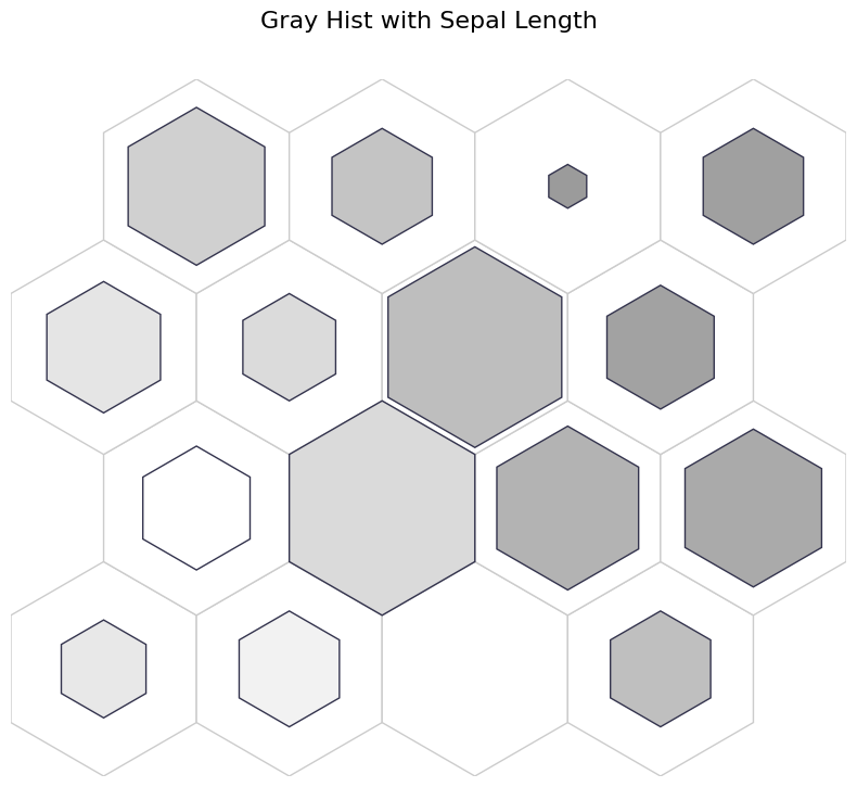
Gray Hist

Gray Hist with continuous data in X

Brigher: Longer

Darker: Shorter

# Visualization
fig, ax, pathces, text = som.plot('gray_hist', data_dict, ind=0)
plt.suptitle("Gray Hist with Sepal Length", fontsize=16)
plt.show()

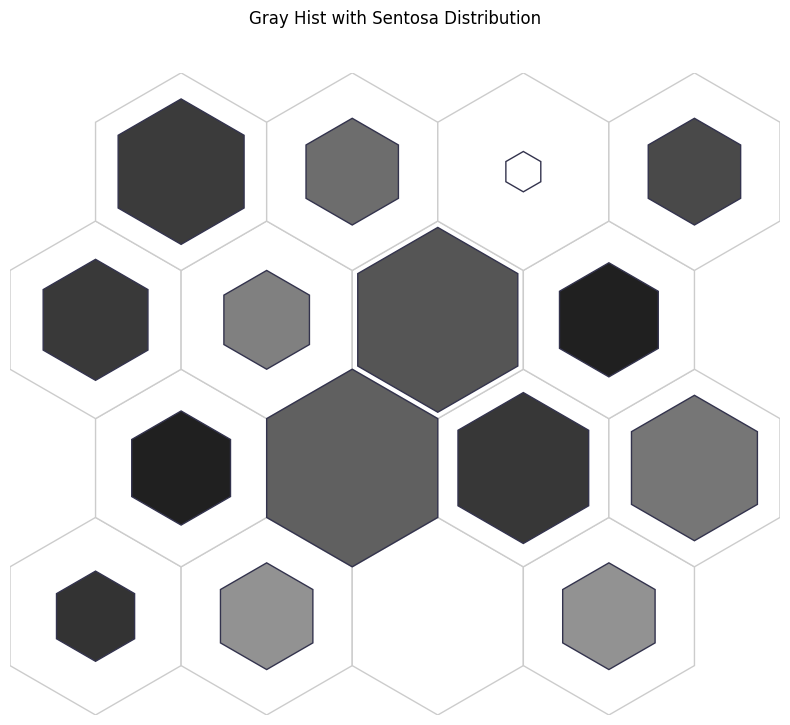
Gray Hist with Caterogrical Variable

Brighter: More Sentosa

Darker: Less Sentosa

fig, ax, pathces, text = som.plot('gray_hist', data_dict, target_class=0)
plt.suptitle("Gray Hist with Sentosa Distribution")
plt.show()

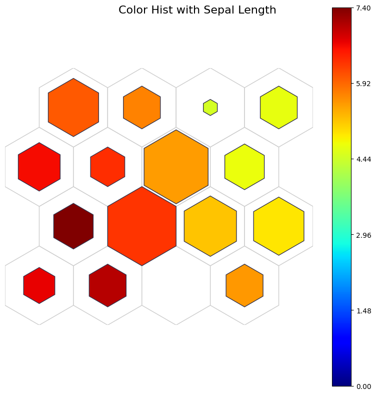
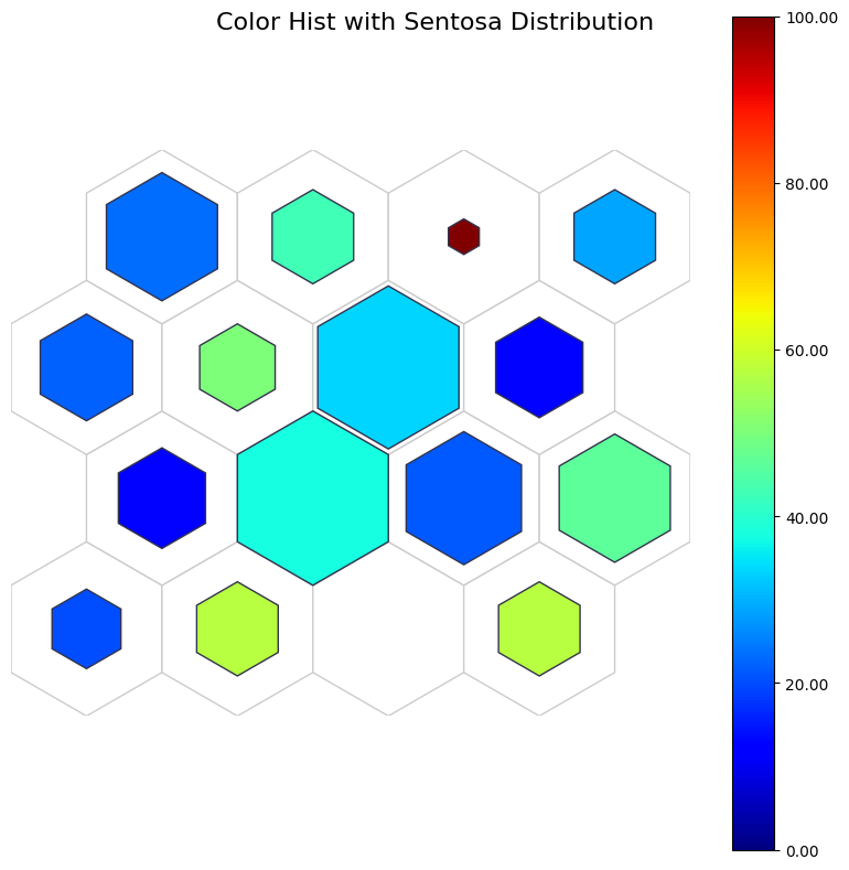
Color Hist

Color Hist with continuous variable

fig, ax, pathces, text, cbar = som.plot('color_hist', data_dict, ind=0)
plt.suptitle("Color Hist with Sepal Length", fontsize=16)
plt.show()

Color Hist with categorical variable

fig, ax, patches, text, cbar = som.plot('color_hist', data_dict, target_class=0)
plt.suptitle("Color Hist with Sentosa Distribution", fontsize=16)
plt.show()

Basic Plots

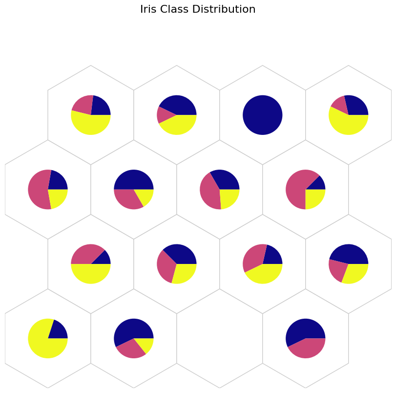
Pie Chart

Blue: Sentosa

Yellow: Virginica

Pink: Vercicolor

fig, ax, h_axes = som.plot("pie", data_dict)
plt.suptitle("Iris Class Distribution", fontsize=16)
plt.show()

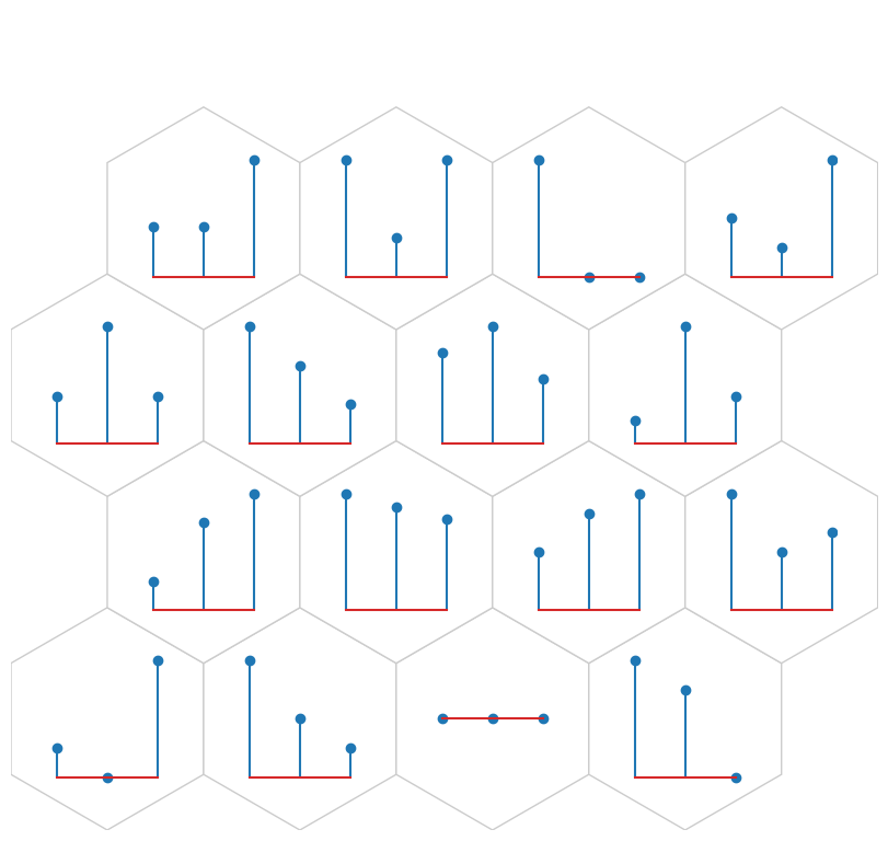
Stem Plot

x: Categories (0: sentosa, 1: versicolor, 2: virginica)

y: count for each class

fig, ax, h_axes = som.plot('stem', data_dict)
plt.show()

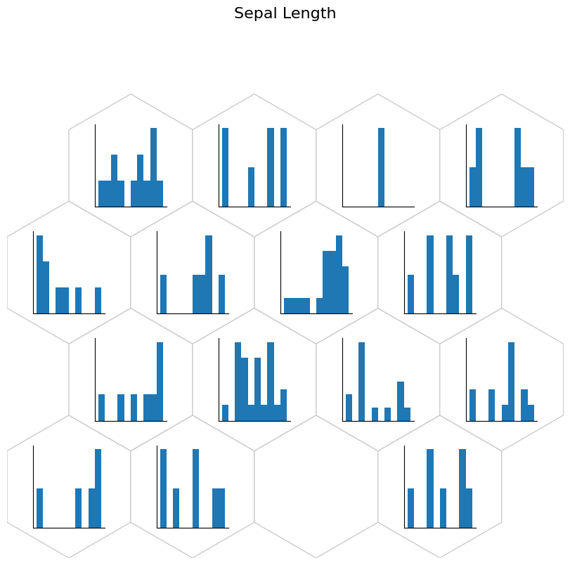
Histogram

fig, ax, h_axes = som.plot('hist', data_dict, ind=0)
plt.suptitle("Sepal Length", fontsize=16)
plt.show()

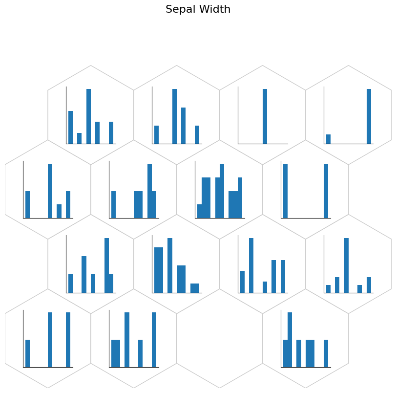
fig, ax, h_axes = som.plot('hist', data_dict, ind=1)
plt.suptitle("Sepal Width", fontsize=16)
plt.show()

Box Plot

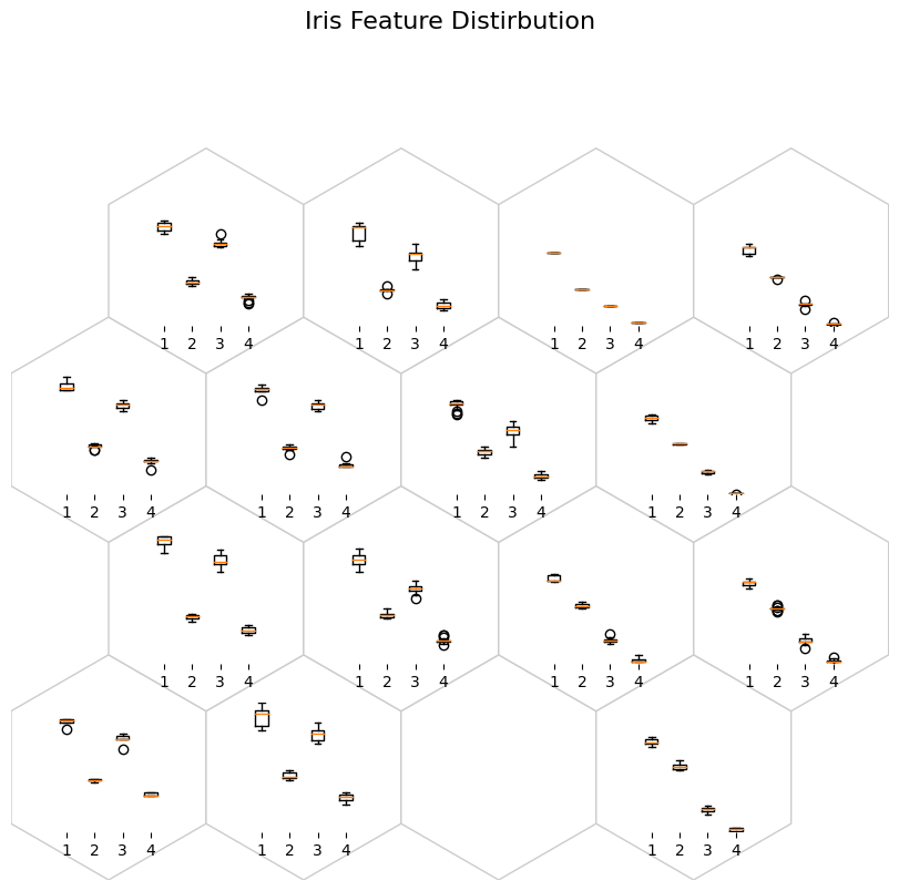
fig, ax, h_axes = som.plot("box", data_dict)
plt.suptitle("Iris Feature Distirbution", fontsize=16)
plt.show()

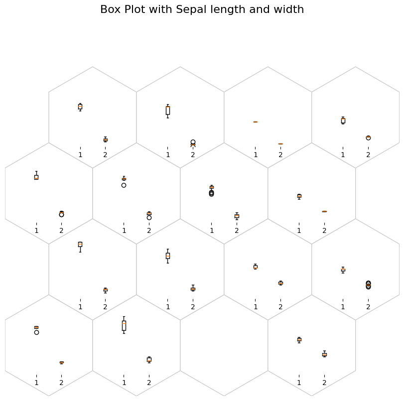
fig, ax, h_axes = som.plot("box", data_dict, ind=[0, 1])
plt.suptitle("Box Plot with Sepal length and width", fontsize=16)
plt.show()

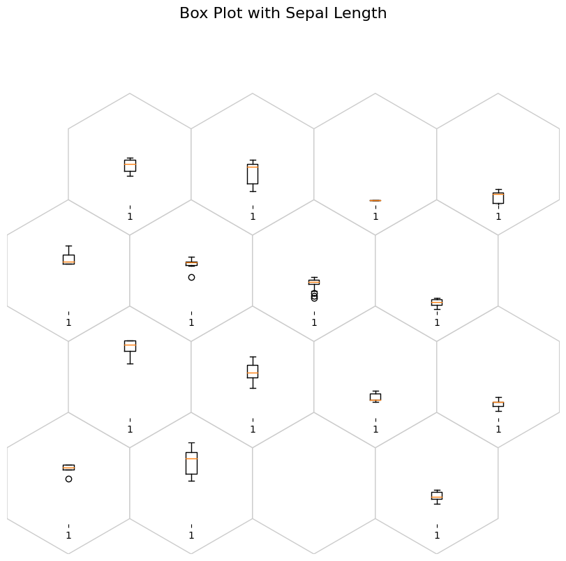
fig, ax, h_axes = som.plot("box", data_dict, ind=0)
plt.suptitle("Box Plot with Sepal Length", fontsize=16)
plt.show()

Violin Plot

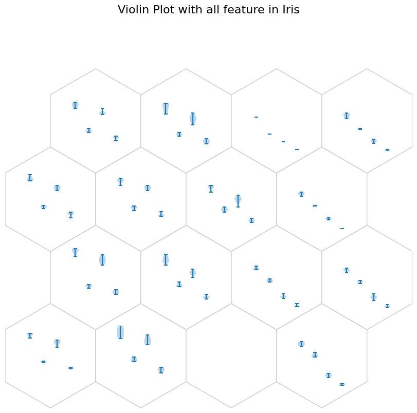
fig, ax, h_axes = som.plot("violin", data_dict)
plt.suptitle("Violin Plot with all feature in Iris", fontsize=16)
plt.show()

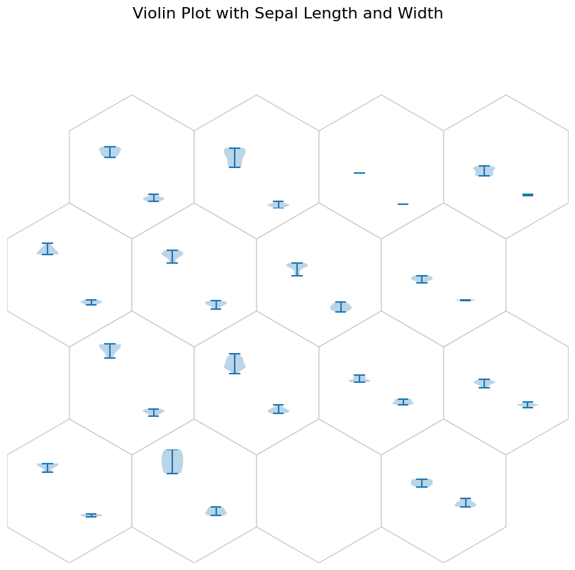
fig, ax, h_axes = som.plot("violin", data_dict, ind=[0, 1])
plt.suptitle("Violin Plot with Sepal Length and Width", fontsize=16)
plt.show()

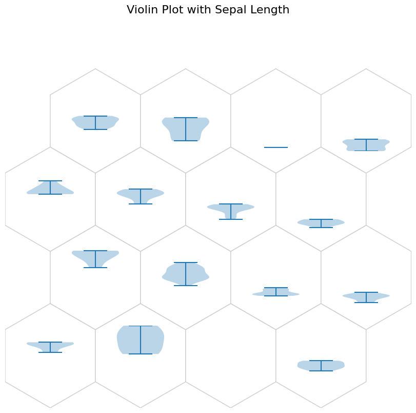
fig, ax, h_axes = som.plot("violin", data_dict, ind=0)
plt.suptitle("Violin Plot with Sepal Length", fontsize=16)
plt.show()

Scatter Plot

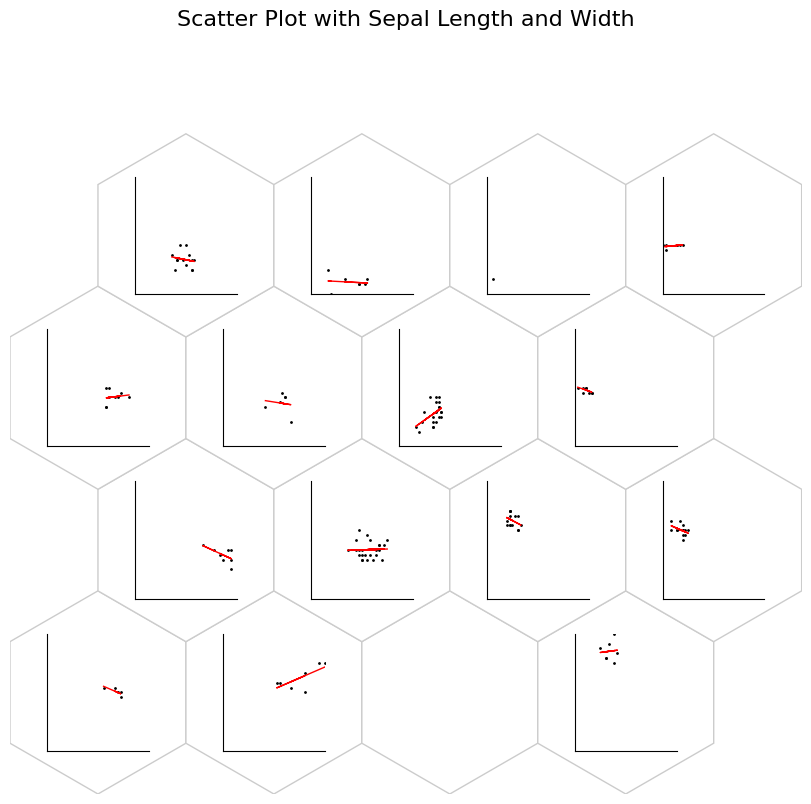
fig, ax, h_axes = som.plot("scatter", data_dict, ind=[0,1])
plt.suptitle("Scatter Plot with Sepal Length and Width", fontsize=16)
plt.show()

/usr/local/lib/python3.10/dist-packages/NNSOM/plots.py:1197: RankWarning: Polyfit may be poorly conditioned
  m, p = np.polyfit(x[neuron], y[neuron], 1)

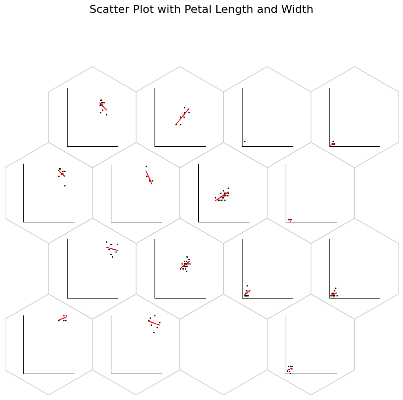
fig, ax, h_axes = som.plot("scatter", data_dict, ind=[2, 3])
plt.suptitle("Scatter Plot with Petal Length and Width", fontsize=16)
plt.show()

/usr/local/lib/python3.10/dist-packages/NNSOM/plots.py:1197: RankWarning: Polyfit may be poorly conditioned
  m, p = np.polyfit(x[neuron], y[neuron], 1)

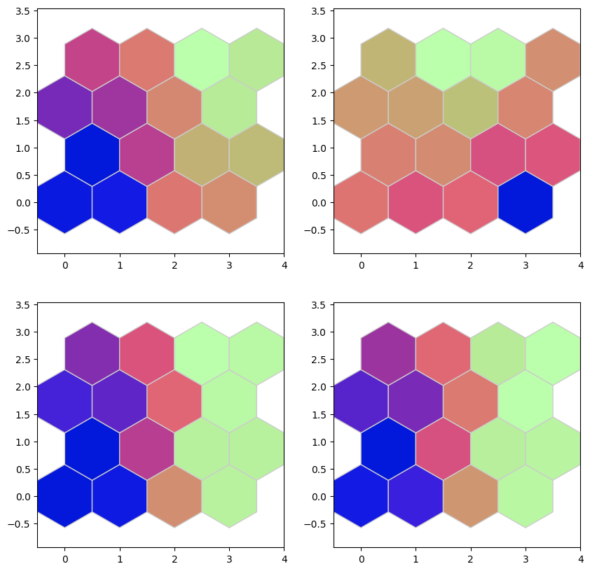
Component Planes

som.plot('component_planes', data_dict)