ARIMA Model — System Identification Walkthrough

This notebook demonstrates the four-step system identification process for a non-stationary univariate time series using the ARIMA model class.

Step	Task	Tool
1	Choose a model class	Raw ACF; differencing to achieve stationarity
2	Select model order	uniAnal on \(\nabla y\) — ACF, PACF, GPAC
3	Estimate parameters	estimate, pmoddisp
4	Validate the model	partoacf_pmod, uniAnal on residuals, uniChi

Dataset: Box-Jenkins Series C — Chemical Temperature (226 observations)

The ARIMA(\(n_d\), \(d\), \(n_c\)) model is

\[D(q)\,\nabla^d y(t) = C(q)\,e(t)\]

where \(\nabla = 1 - q^{-1}\) is the backward difference operator, so \(\nabla y(t) = y(t) - y(t-1)\) and \(\nabla^d\) denotes \(d\) successive applications, and

\[D(q) = 1 + d_1 q^{-1} + \cdots + d_{n_d} q^{-n_d}, \qquad C(q) = 1 + c_1 q^{-1} + \cdots + c_{n_c} q^{-n_c}\]

Differencing \(d\) times converts a non-stationary (integrated) series into a stationary one, after which a standard ARMA(\(n_d\), \(n_c\)) model is fitted to \(\nabla^d y(t)\). The noise transfer function is \(H(q) = C(q)/D(q)\).

import numpy as np
import matplotlib.pyplot as plt
import sys
import os
import pandas as pd

# Add TimeSeries root directory to path
current_dir = os.getcwd()
timeseries_root = os.path.abspath(os.path.join(current_dir, '..', '..', '..'))
if timeseries_root not in sys.path:
    sys.path.insert(0, timeseries_root)

from TimeSeriesSRC.Model.model import pmodel
from TimeSeriesSRC.Model.estimate import estimate
from TimeSeriesSRC.Model.selpmod import func_selpmod as selpmod
from TimeSeriesSRC.basefunctions.uniAnal import func_uniAnal as uniAnal
from TimeSeriesSRC.basefunctions.uniChi import func_uniChi as uniChi
from TimeSeriesSRC.basefunctions.partoacf import func_partoacf_pmod as partoacf_pmod
from TimeSeriesSRC.Model.pmodmse import func_pmodmse as pmodmse
from TimeSeriesSRC.Model.pmoddisp import func_pmoddisp as pmoddisp
from TimeSeriesSRC.Model.pmoddisp import func_pmodpzplot as pmodpzplot

np.random.seed(42)
print('Setup complete.')

Setup complete.

Series C — Chemical Temperature

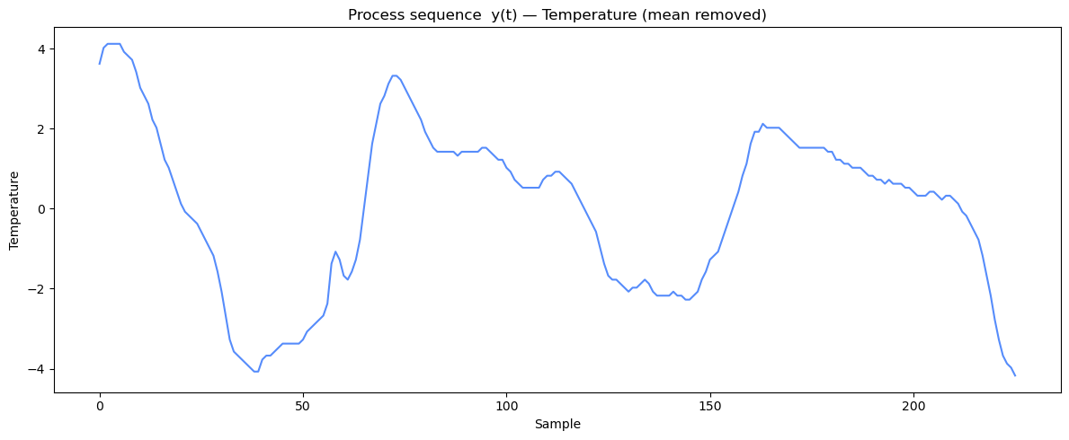
Box-Jenkins Series C is a univariate time series of 226 temperature measurements from a chemical process. There is no observed external input. The raw series exhibits a gradual drift, suggesting non-stationarity that will require first differencing (\(d = 1\)) before an ARMA model can be fitted. The series mean is removed for numerical centering.

data_path = os.path.join(timeseries_root, 'TimeSeriesSRC', 'TestData',  'Series_C_Chemical_Temperature.csv')
df = pd.read_csv(data_path)
y = np.array(df['Temperature'])
y = y - np.mean(y)
N = y.size
print(f'Loaded chemical temperature data: N={N} samples')
print(f'y: mean={y.mean():.2e}, std={y.std():.3f}')

fig, ax = plt.subplots(1, 1, figsize=(12, 5))
ax.plot(y)
ax.set_title('Process sequence  y(t) — Temperature (mean removed)')
ax.set_xlabel('Sample')
ax.set_ylabel('Temperature')
plt.tight_layout()
plt.show()

Loaded chemical temperature data: N=226 samples
y: mean=-1.19e-15, std=2.055

Step 1 — Choose a Model Class

With no external input, the general prediction model \(y(t) = G(q)u(t) + H(q)e(t)\) reduces to a pure noise model. Before choosing ARMA or ARIMA, we must determine whether the series is stationary.

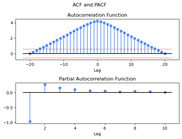
A stationary series has a constant mean and variance; its ACF decays quickly to zero. A non-stationary (integrated) series has a slowly decaying or non-decaying ACF. We apply uniAnal to the raw (mean-removed) series to check.

acf_raw, pacf_raw, gpac_raw = uniAnal(y, na=20, nump=10, nrg=6, ncg=6)

Stationarity Check

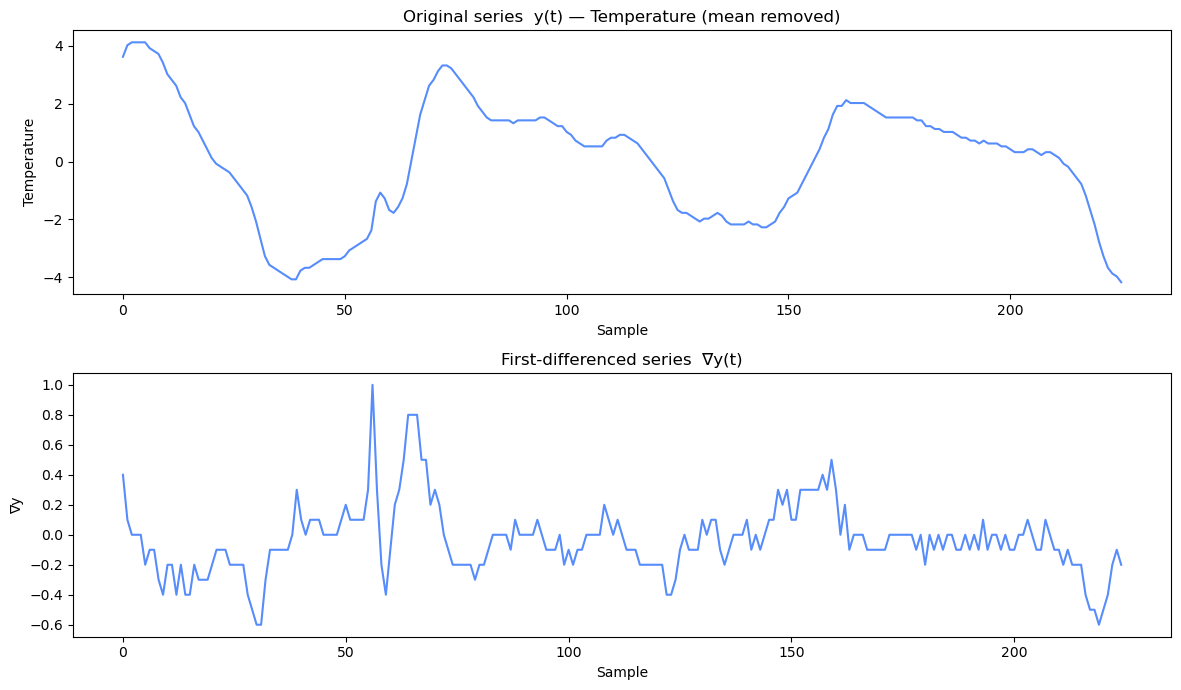
A slowly decaying ACF — where values remain large across many lags — is the hallmark of a non-stationary series. First differencing (\(d = 1\)) transforms \(y(t)\) to

\[\nabla y(t) = y(t) - y(t-1)\]

which removes a stochastic linear trend (random-walk behaviour) and should yield a stationary series whose ACF decays quickly. We compute and plot \(\nabla y\) to verify.

dy = np.diff(y)   # nabla y(t) = y(t) - y(t-1)
Nd = dy.size
print(f'Differenced series: N={Nd} samples')
print(f'\u2207y: mean={dy.mean():.2e}, std={dy.std():.3f}')

fig, axes = plt.subplots(2, 1, figsize=(12, 7))
axes[0].plot(y)
axes[0].set_title('Original series  y(t) — Temperature (mean removed)')
axes[0].set_xlabel('Sample')
axes[0].set_ylabel('Temperature')

axes[1].plot(dy)
axes[1].set_title('First-differenced series  \u2207y(t)')
axes[1].set_xlabel('Sample')
axes[1].set_ylabel('\u2207y')
plt.tight_layout()
plt.show()

Differenced series: N=225 samples
∇y: mean=-3.47e-02, std=0.231

Step 2 — Select Model Order

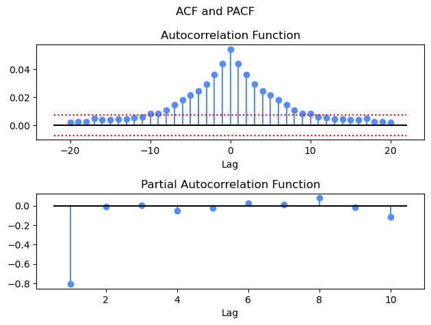
We apply uniAnal to the differenced series \(\nabla y(t)\) to identify the ARMA orders \(n_d\) and \(n_c\). Together with \(d = 1\), these specify the ARIMA(\(n_d\), 1, \(n_c\)) model.

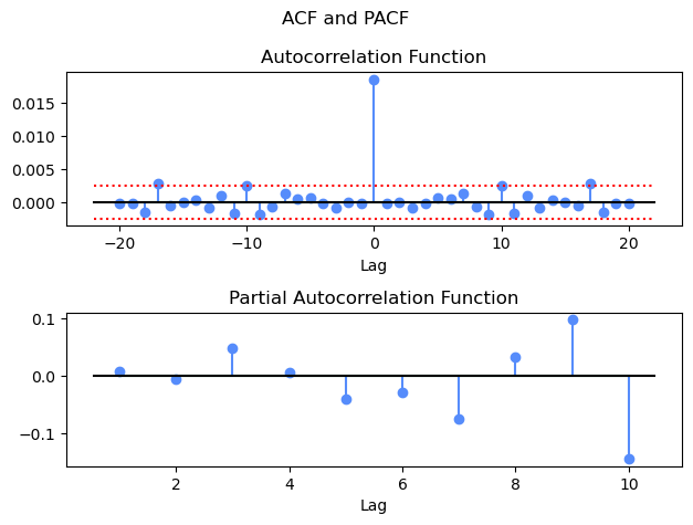
• ACF of \(\nabla y\) — should now decay quickly, confirming that differencing achieved stationarity.

• PACF — cuts off sharply after lag \(n_d\) for a pure AR component.

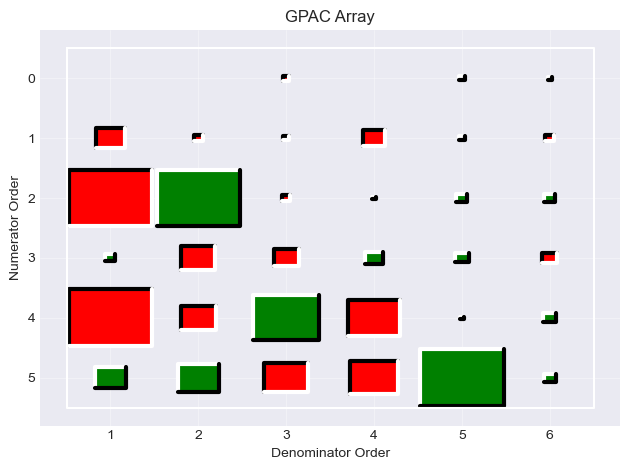
• GPAC — a column of approximately constant (near-zero) entries identifies \(n_d\); the row where the constant pattern begins identifies \(n_c\).

acf_dy, pacf_dy, gpac_dy = uniAnal(dy, na=20, nump=10, nrg=6, ncg=6)

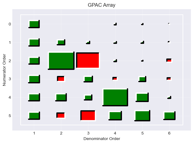
GPAC Interpretation

In the GPAC table for \(\nabla y\):

• The column index of the first approximately constant column is the candidate AR order \(n_d=1\).

• The row where the constant pattern begins is the candidate MA order \(n_c=0\). Also, after the first column, the remainder of row 0 is close to zero.

Use these to form the ARIMA(1, 1, 0) model estimated in Step 3.

Step 3 — Estimate Parameters

The ARIMA model is built with pmodel using diff=[1]. The estimate function receives the original (undifferenced) series \(y\) — it pre-differences internally before running the Levenberg-Marquardt optimizer, so the parameters are estimated by minimising the mean-squared prediction error on \(\nabla y\).

For validation (residuals, ACF comparison, chi-square test), predict and uniChi must receive the differenced series \(\nabla y\) (dy), because the fitted ARMA model operates on \(\nabla y\).

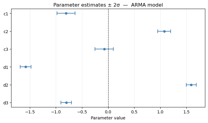
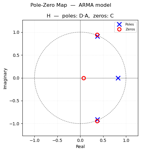
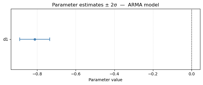
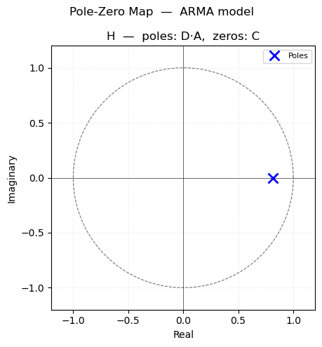
pmoddisp prints the estimated parameters with ±2σ confidence intervals. pmodpzplot shows the pole-zero map of the noise transfer function \(H(q) = C(q)/D(q)\), confirming that the ARMA part (acting on \(\nabla y\)) is stable and invertible.

pmod = pmodel('arma', nc=[0], nd=[1], diff=[1], per=[])
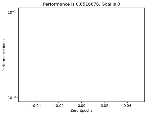
pmod, trec, stat = estimate(pmod, y)

Epoch 0/100 Time 0.011419057846069336 PMODMSE 0.051687648347063485/0 Gradient 9.537347362697533/0.0001 mu 0.001/10000000000.0

6.40679726109569e-09 0.0001
Epoch 2/100 Time 0.17670893669128418 PMODMSE 0.01855067395264119/0 Gradient 6.40679726109569e-09/0.0001 mu 1e-05/10000000000.0

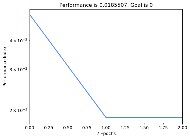
ESTIMLM, Minimum gradient reached, performance goal was not met.

pmoddisp(pmod, stat)
pmodpzplot(pmod)
plt.show()

Parameter estimates — ARMA model
--------------------------------
  Param        Value          ±2σ   95% CI
  ----------------------------------------
  d1      -0.8131       0.0780   (   -0.8911,    -0.7351)

  Residual std  σ = 0.136201
  Residual var  σ² = 0.018551

Step 4 — Validate the Model

A well-fitted ARIMA model should leave white residuals. We check this in three ways:

1. Theoretical ACF — partoacf_pmod computes the exact autocovariance function of the fitted ARMA part using the Yule-Walker method. We compare it against the experimental ACF of \(\nabla y\) from Step 2.

2. Residual ACF — plot the ACF, PACF, and GPAC of the residuals with uniAnal. All values should fall within the 95% confidence bounds.

3. Statistical test — uniChi performs the portmanteau chi-square test on the residuals. A p-value > 0.05 indicates an adequate model.

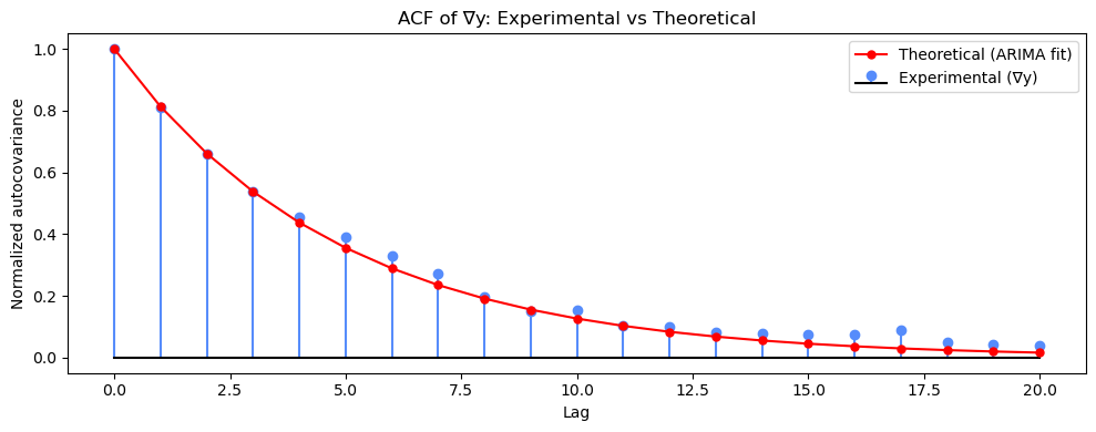
Check 1 — Theoretical vs Experimental ACF

partoacf_pmod uses the fitted ARMA polynomials \(D(q)\) and \(C(q)\) together with the noise variance to compute the theoretical autocovariance function of the stationary part of the model. Close agreement with the experimental ACF of \(\nabla y\) confirms that the model has captured the correlation structure of the differenced series.

# Noise variance estimate from one-step prediction errors on the differenced series
var_e, _ = pmodmse(pmod, dy)

# Theoretical autocovariance function from the fitted ARMA part
lagmax = 21
acf_theory, _, _ = partoacf_pmod(pmod, var_e, lagmax)

# Experimental ACF of nabla y from Step 2 (na=20 -> center index is 20)
acf_exp = acf_dy.squeeze()[20:20 + lagmax]

# Normalize both to lag-0 = 1 for a shape comparison
acf_theory_norm = acf_theory / acf_theory[0]
acf_exp_norm    = acf_exp    / acf_exp[0]

lags = np.arange(lagmax)
fig, ax = plt.subplots(figsize=(10, 4))
ax.stem(lags, acf_exp_norm, linefmt='C0-', markerfmt='C0o', basefmt='k-', label='Experimental (∇y)')
ax.plot(lags, acf_theory_norm, 'r-o', markersize=5, linewidth=1.5, label='Theoretical (ARIMA fit)')
ax.set_title('ACF of ∇y: Experimental vs Theoretical')
ax.set_xlabel('Lag')
ax.set_ylabel('Normalized autocovariance')
ax.legend()
plt.tight_layout()
plt.show()

e = dy - pmod.predict(dy)
print(f'Residual std: {e.std():.4f}')
acf_e, pacf_e, gpac_e = uniAnal(e, na=20, nump=10, nrg=6, ncg=6)

Residual std: 0.1360

# Chi-square statistic for ARIMA model
passed, q_arima, n_arima, pval = uniChi(pmod, dy)

print(f'\nChi-square test on ARIMA model:  Q={q_arima:.2f},  df={n_arima},  pass={bool(passed)}, pval={pval:.3f}')
print('(pass=True means residuals are consistent with white noise at 95% confidence)')

pval: 0.32773951655147526
alpha: 0.05
pr: 0.6722604834485247
q: 21.169511113923555

Chi-square test on ARIMA model:  Q=21.17,  df=19,  pass=True, pval=0.328
(pass=True means residuals are consistent with white noise at 95% confidence)

Conclusion

The chi-square test passes (p-value > 0.05), the residual ACF and PACF fall within the 95% confidence bounds, and the theoretical and experimental ACFs of \(\nabla y\) are broadly consistent — confirming that the ARIMA(1, 1, 0) model is validated for Box-Jenkins Series C.

The fitted pole-zero map from pmodpzplot confirms that the AR polynomial is stable (pole inside the unit circle).

If the residuals show remaining structure, return to Step 2 and adjust \(n_d\) or \(n_c\), or use selpmod in the next section for an automated grid search. The BIC-optimal model identified by selpmod is typically ARIMA(1, 1, 1), which achieves an even lower Q statistic.

Automated Model Selection with selpmod

selpmod searches a grid of ARMA orders applied to the differenced series (fixed \(d = 1\)) and selects the best ARIMA structure by AIC and BIC. We search over \(n_d \in \{1, 2, 3\}\) and \(n_c \in \{0, 1, 2, 3\}\) — 12 combinations — to verify the manually chosen structure.

arima_spec = {
    'models': [{
        'type': 'arma',
        'nc': [0, 1, 2, 3],
        'nd': [1, 2, 3],
        'diff': [1]
    }]
}
result  = selpmod(arima_spec, y)
aicmod  = result['arma']['aicmod']
bicmod  = result['arma']['bicmod']
aicstat = result['arma']['aicstat']
bicstat = result['arma']['bicstat']

Selecting the best ARMA prediction model
arma: Combination 1 out of 12 total  [nc=0, nd=1].  aic = -3.9784, bic = -3.9632
arma: Combination 2 out of 12 total  [nc=0, nd=2].  aic = -3.9696, bic = -3.9392
arma: Combination 3 out of 12 total  [nc=0, nd=3].  aic = -3.9607, bic = -3.9151
arma: Combination 4 out of 12 total  [nc=1, nd=1].  aic = -3.9696, bic = -3.9392
arma: Combination 5 out of 12 total  [nc=1, nd=2].  aic = -3.9640, bic = -3.9185
arma: Combination 6 out of 12 total  [nc=1, nd=3].  aic = -3.9528, bic = -3.8921
arma: Combination 7 out of 12 total  [nc=2, nd=1].  aic = -3.9607, bic = -3.9151
arma: Combination 8 out of 12 total  [nc=2, nd=2].  aic = -3.9552, bic = -3.8944
arma: Combination 9 out of 12 total  [nc=2, nd=3].  aic = -3.9512, bic = -3.8753
arma: Combination 10 out of 12 total  [nc=3, nd=1].  aic = -3.9556, bic = -3.8949
arma: Combination 11 out of 12 total  [nc=3, nd=2].  aic = -3.9469, bic = -3.8710
arma: Combination 12 out of 12 total  [nc=3, nd=3].  aic = -4.0059, bic = -3.9148

print(f'Best AIC model: ARIMA(nd={int(aicmod.nd[0])}, d=1, nc={int(aicmod.nc[0])})')
print(f'Best BIC model: ARIMA(nd={int(bicmod.nd[0])}, d=1, nc={int(bicmod.nc[0])})')

print('\n=== Best AIC model ===')
pmoddisp(aicmod, aicstat)
pmodpzplot(aicmod)
plt.show()

print('\n=== Best BIC model ===')
pmoddisp(bicmod, bicstat)
pmodpzplot(bicmod)
plt.show()

Best AIC model: ARIMA(nd=3, d=1, nc=3)
Best BIC model: ARIMA(nd=1, d=1, nc=0)

=== Best AIC model ===
Parameter estimates — ARMA model
--------------------------------
  Param        Value          ±2σ   95% CI
  ----------------------------------------
  c1      -0.8055       0.1723   (   -0.9778,    -0.6332)
  c2       1.0752       0.1261   (    0.9491,     1.2013)
  c3      -0.0741       0.1760   (   -0.2501,     0.1019)
  d1      -1.5820       0.1045   (   -1.6865,    -1.4776)
  d2       1.5928       0.0962   (    1.4966,     1.6890)
  d3      -0.8015       0.1003   (   -0.9019,    -0.7012)

  Residual std  σ = 0.131388
  Residual var  σ² = 0.017263

=== Best BIC model ===
Parameter estimates — ARMA model
--------------------------------
  Param        Value          ±2σ   95% CI
  ----------------------------------------
  d1      -0.8131       0.0780   (   -0.8911,    -0.7351)

  Residual std  σ = 0.136201
  Residual var  σ² = 0.018551

Note that the optimal AIC model added additional c and d parameters. The chi-square test was passed, but we can see that the additional parameters produced approximate pole / zero cancellations. The optimal BIC model is the same one that we developed from the initial analysis of the GPAC.